I have been working on this Wendy Davis data for a long time, but realized I had not caught you guys up to speed with it in a while. Here is what I have been doing for the past month with the data.

First, I found the data, thanks to the amazing Kelly Blanchat, who discovered it in a database at the University of North Texas.

Phase #1: JSON to CSV

Then, after I agonized over what to do with JSON files for a really long time. I found a reader for them called Sublime Text, but had trouble pasting that data accurately into a spreadsheet. Then, when I found out how to do that, I had to figure out how to make the data nice and neat, getting rid of all the punctuation that wasn’t needed in the file I would be using for Gephi. I did some of this by hand, and then found a site called Json-to-CSV that would do some of this for you. At first, this program seemed great, but then I realized that my whole file was too big to fit. The progress bar was forever stuck about an inch away from the end, but would not finish. I began to think about cutting down the data somehow, but couldn’t figure out how I would get a representative sample. Furthermore, because (as I figured out pretty quickly) JSON data do not have all the information fields predictably in the same place every time (like the way they show up in Excel) I could not do the data set in pieces, because the program could very well put the fields in different places every time, if it was working with what it considered to be more than one set of data. What I ended up doing was upgrading to their pro edition, which was like $5. In the end, however, I realized that it was the browser that was the problem. It would stall every time I tried to load the data, even though the program itself could technically handle the extra memory. In the end, I pasted the JSON data into several different spreadsheet files. Then, I cut out the irrelevant data leaving only the tweet, hashtag, and location, and pasted them all into the same spreadsheet to get ready for Gephi. Then I finally got a useful CSV.

Phase #2: Gephi

After that, I began the long haul of learning how to use Gephi. I imported my data files, which were constructed to model the relationships between the central node “I Stand with Wendy” and every other hashtag that was used in the dataset. As there weren’t that many other hashtags that were used anywhere near as frequently, it really didn’t make sense to me to model the relationships among these other hashtags. Though Margaret, the librarian who ran the library’s Analyzing Data workshop demonstrated Gephi for us briefly, I hadn’t really played around with it before. It took me a while to figure out how to do anything, because I am a very tactile learner. I kind of have to do things to understand them, and cannot get much from reading instructions, though watching how-to videos sometimes helps. At any rate, it took me a while. The hardest thing to figure out was that there didn’t seem to be any way to restore the graph to its original look after you changed the format. Also, I kept zooming in or out, and sometimes, even when I would center on the graph and zoom back out or in again, I couldn’t find the graph again.

Phase #3: The Great Fuck-Up

After a while, though, I got  something that looked pretty great to me, though because I saved it as a PDF (I didn’t yet know how to work the screen shot feature), it doesn’t look quite as great to me as it did at the time. The big developments at this stage were the decision to use force atlas, mostly because it looked best, and the decision to color code the nodes. I made the nodes blue and the edges red, creating a visualization that looked morbidly but aptly considering the subject like blood oozing, or like Republican nodes shooting from a Democratic center, simulating the geography of Texas itself.

I had taken off the labels to make the visualization clearer, and then decided to put them back on. That was when I noticed something strange. The only node that was substantially bigger than the rest (but smaller than #IStandwithWendy), was #StanleyCup. I thought it was strange that a bunch of abortion rights activists would also go crazy for the Stanley Cup, but I wasn’t discounting the possibility yet. I went back and looked at my original file, and found that the hashtag had only been used once, and my blood ran cold. Apparently, when making the edges file, I had left out the hashtag “American,” probably seeing how similar it was to “America” and thinking I already had it, therefore misaligning the edge weights, putting #StanleyCup one field further up where #StandwithWendy (the imperative as opposed to the declarative) should have been.

Eventually, I was able to laugh about this, but at the time I was pretty pissed off. There probably was a way to make these files through Gephi rather than putting in the weights and assigning the nodes numbers myself that would have precluded me from making such a mistake. I really am the kind of person who has to make mistakes to learn, though. And I learned a lot that day.

Phase #4: Something Kind of Pretty and Not Wrong

After a few more hours of work, I had something that looked a lot better (and was actually accurate this time to boot). Learning how to make the size of the nodes correlate to how many times each one was used really helped make the graph both more meaningful and visually appealing. Learning how to play around with the label font size also helped a lot, making the words correlate to node size as well, and playing around with the size so I could make as many labels as possible visible while still not having so many that viewers couldn’t read them. And I learned how to use the screen shot function, so I could take a decent picture of it. Finally, though I just had to take the labels off because you still couldn’t see anything. For your information, though, some of the most frequently tweeted hashtags (other than “Istandwithwendy”) were “txlege,” “texlege,” “sb5” (the name of the bill), and “standwithwendy.”  Unfortunately, the screen shot function does not do color, or if it doesn’t I couldn’t figure it out. Here it is:

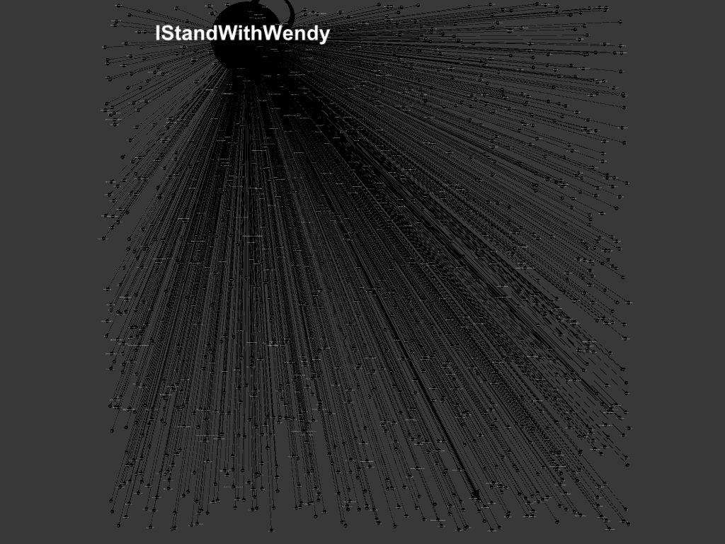
I wasn’t entirely happy with this visualization, because I am not sure it really shows very much. It shows that “IStandwithWendy” is the most frequently used hashtag, and shows that, other than that, most hashtags weren’t used that often (except for the few I just mentioned). It doesn’t show some of the interesting nuances of the dataset, like the fact that some pro-life people were tweeting “IStandwithWendy” sarcastically, and some people were tweeting “IStandwithWendy” as in the restaurant as a joke (albeit one in pretty poor taste).

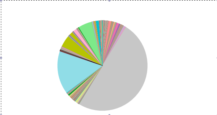
Phase #5: Tableau Public Pie Chart

Because of this drawback, I decided to make a pie chart on Tableau Public that would at least show the relative frequencies of some of the hashtags a little more clearly. I was having a bit of trouble with their export function, so I just took a screenshot, which doesn’t allow you to interact with the graph like you would have bee able to. Here it is:

I really want to continue with this project and do the geographic map of tweets that I wanted to        do originally. Thanks, everyone for reading, and for all of the ways in which you have helped me learn DH skills this semester! Have a great holiday!